Everyday Radio Telescope
No journal publication or individual INSPIRE record has been confirmed for this paper. The original arXiv article is the primary source for this summary.
Motivation and setup
Radio astronomy offers a way to study astronomical objects beyond visible light, but the equipment can appear inaccessible to an undergraduate laboratory or amateur group. This project develops an affordable experiment from commercially available satellite-television components. Its aim is educational as well as observational: to connect receiving electronics, digitization, calibration, statistical noise, and astronomical interpretation in a working instrument.
The telescope operates near 11.2 GHz. A parabolic dish concentrates incoming radiation onto a low-noise block receiver, or LNB. A satellite finder acts as a square-law detector, producing a signal related to received intensity. An Arduino Uno digitizes the output with a ten-bit analog-to-digital converter at ten samples per second. A set-top box supplies power, and a Python pipeline records and displays the measurements. The instrument is an intensity-measuring system; the paper does not present it as an imaging array or a frequency-resolving radio spectrometer.
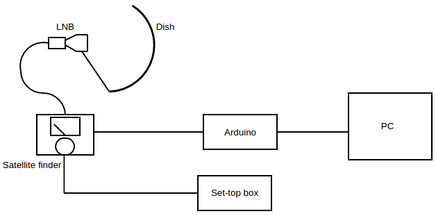
The Sun supplies a strong first target. Geostationary satellites provide reference signals for calibration, and sky observations away from a target supply the background. Pointing is manual, using predicted altitude and azimuth. For satellite calibration, rotating the LNB aligns its receiving element with the transmitted polarization and maximizes the detected signal. This makes the polarization response part of the experiment rather than an invisible correction.
The calibration begins with the Friis transmission relation, reproduced from equation (2):
\[ \frac{P_r}{P_t}=G_tG_r\left(\frac{\lambda}{4\pi R}\right)^2. \]
Here the received and transmitted powers are \(P_r\) and \(P_t\), the antenna gains are \(G_r\) and \(G_t\), \(R\) is the satellite distance, and \(\lambda\) is the observing wavelength. Satellite equivalent isotropically radiated power combines the transmitter power and gain, allowing the received reference power to be estimated from accessible satellite information.
Construction and main results
Converting a voltage change into an astronomical measurement requires both the detector calibration and an estimate of the effective collecting area. The receiving gain is related to dish diameter and aperture efficiency by equation (4):
\[ G_r=\eta_A\left(\frac{\pi d}{\lambda}\right)^2. \]
The aperture efficiency \(\eta_A\) accounts for the difference between geometric dish area and effective collecting area. The appendix uses this information to turn the measured satellite voltage above background into a power scale. The solar signal is then calibrated relative to the satellite observation, preferably taken close in time so that instrumental conditions are comparable.
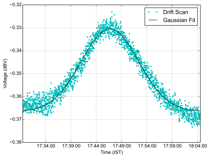
A drift scan holds the antenna pointing fixed while the sky moves through its beam. Fitting the solar transit with a Gaussian provides a beam-width estimate as well as a recognizable source detection. The paper reports beam widths of approximately \(3.4\)–\(3.5\) degrees, with the tabulated fits giving \(3.357\pm0.021\) and \(3.501\pm0.007\) degrees. These measurements agree with the approximate beam width expected for the instrument. The broad beam makes source acquisition forgiving, while also limiting angular resolution.
The appendix next converts received power to flux density, including the single-polarization response and the difference between the satellite’s transmitted bandwidth and the receiver’s solar-observation bandwidth. Dividing the flux by the solar solid angle gives intensity. Assuming thermal radiation in the Rayleigh–Jeans regime, the final temperature relation shown in Appendix A, unnumbered, is
\[ T=\frac{I\lambda^2}{2K_B}=10078\,K. \]
This is the paper’s worked calibration example, with \(I\) the inferred intensity and \(K_B\) Boltzmann’s constant. The two reported solar brightness temperatures are 10078 K and 10136 K, with quoted uncertainties of 295 K and 324 K. Brightness temperature describes the observed intensity at the operating frequency; it should not be confused with a direct measurement of the Sun’s photospheric temperature.
Sensitivity can improve by averaging longer. The relevant relation is the radiometer equation, equation (1):
\[ \sigma_T\propto\frac{1}{\sqrt{\tau\Delta\nu_{RF}}}. \]
The output fluctuation \(\sigma_T\) decreases as integration time \(\tau\) or receiver bandwidth \(\Delta\nu_{RF}\) increases, under the assumptions behind that noise model. Increasing integration from one second to sixty seconds enabled the reported drift-scan detections of Saturn and a Galactic-arm crossing. The Saturn detection has a reported signal-to-noise ratio of three, with transit timing checked against the predicted sky motion.
Interpretation and limits
This experiment brings several normally separate classroom topics into one measurement. The receiving chain illustrates amplification and detection; the digitizer turns a continuous voltage into a sampled series; calibration connects the output to physical units; and drift scans connect time-domain structure to the sky. A simple setup can therefore teach the reasoning behind a radio measurement without requiring a large professional observatory.
The paper also investigates noise rather than treating every fluctuation as astronomical. Comparing ordinary sky measurements with observations made while the LNB is shielded helps distinguish system-generated features. Fourier analysis shows instrumental structure in the time series, including a feature around half a hertz. Ambient temperature changes also track the detector voltage: the reported correlation coefficient is 0.98. Longer averaging alone cannot remove a drifting calibration or establish that every feature comes from a celestial source.
The reported weaker-source detections should be read with those limitations in mind. Their interpretation relies on timing, pointing, background behavior, and modest signal-to-noise, rather than high-resolution imaging. The solar calibration assumes thermal emission, an aperture efficiency, published satellite powers, and a linear extrapolation between the satellite and solar bandwidths. Those assumptions explain what the quoted temperature estimates mean and where systematic uncertainty can enter.
There is also a dimensional inconsistency within the original article: the setup description gives a 68 cm dish, whereas the appendix’s numerical gain substitution uses 0.71 m. This summary preserves the source equations and reported measurements without silently harmonizing those inputs. The original paper remains the reference for reproducing the experiment and evaluating its calibration in detail.
Source: arXiv:1601.02982, sections II–V and Appendix A; equations (1), (2), and (4), the unnumbered temperature relation, and original Figures 1 and 4. The first arXiv submission is from 2016; the automatically generated date in the HTML rendering is not used as the publication year.
Related: Research overview · All publications and talks.